Effect modificationWhat If: Chapter 4Elena Dudukina2020-11-261 / 43

Definition of the effect modification

The causal effect changes with the characteristics of the population under study

greek_gods_po <- tibble::tribble(
  ~greek, ~V, ~Y_a0, ~Y_a1,
  "Rheia", 1, 0, 1,
  "Demeter", 1, 0, 0,
  "Hestia", 1, 0, 0,
  "Hera", 1, 0, 0, 
  "Artemis", 1, 1, 1,
  "Leto", 1, 0, 1,
  "Athena", 1, 1, 1,
  "Aphrodite", 1, 0, 1,
  "Persephone", 1, 1, 1,
  "Hebe", 1, 1, 0,
  "Kronos", 0, 1, 0,
  "Hades", 0, 0, 0,
  "Poseidon", 0, 1, 0,
  "Zeus", 0, 0, 1, 
  "Apollo", 0, 1, 0,
  "Ares", 0, 1, 1,
  "Hephaestus", 0, 0, 1, 
  "Cyclope", 0, 0, 1,
  "Hermes", 0, 1, 0,
  "Dionysus", 0, 1, 0
)

2 / 43

Definition of the effect modification

# had we known counterfactual outcomes
greek_gods_po %>% 
  count(Y_a0)

## # A tibble: 2 x 2
##    Y_a0     n
##   <dbl> <int>
## 1     0    10
## 2     1    10

greek_gods_po %>% 
  count(Y_a1)

## # A tibble: 2 x 2
##    Y_a1     n
##   <dbl> <int>
## 1     0    10
## 2     1    10

$P r [Y^{a = 1} = 1] - P r [Y^{a = 0} = 1]$ = 0
$\frac{P r [Y^{a = 1} = 1]}{P r [Y^{a = 0} = 1]}$ = 1

3 / 43

What is the average causal effect of A on Y in women and in men?Pr[Ya=1=1|V=1]Pr[Ya=1=1|V=1] - Pr[Ya=0=1|V=1]Pr[Ya=0=1|V=1]
Pr[Ya=1=1|V=0]Pr[Ya=1=1|V=0] - Pr[Ya=0=1|V=0]Pr[Ya=0=1|V=0]
4 / 43

What is the average causal effect of A on Y in women and in men?

$P r [Y^{a = 1} = 1 | V = 1]$ - $P r [Y^{a = 0} = 1 | V = 1]$
$P r [Y^{a = 1} = 1 | V = 0]$ - $P r [Y^{a = 0} = 1 | V = 0]$
$\frac{P r [Y^{a = 1} = 1 | V = 1]}{P r [Y^{a = 0} = 1 | V = 1]}$
$\frac{P r [Y^{a = 1} = 1 | V = 0]}{P r [Y^{a = 0} = 1 | V = 0]}$

4 / 43

What is the average causal effect of A on Y in women and in men?

$P r [Y^{a = 1} = 1 | V = 1]$ - $P r [Y^{a = 0} = 1 | V = 1]$
$P r [Y^{a = 1} = 1 | V = 0]$ - $P r [Y^{a = 0} = 1 | V = 0]$
$\frac{P r [Y^{a = 1} = 1 | V = 1]}{P r [Y^{a = 0} = 1 | V = 1]}$
$\frac{P r [Y^{a = 1} = 1 | V = 0]}{P r [Y^{a = 0} = 1 | V = 0]}$

## # A tibble: 2 x 6
## # Groups:   V [2]
##       V label risk_Y_a1 risk_Y_a0    RR     RD
##   <dbl> <chr>     <dbl>     <dbl> <dbl>  <dbl>
## 1     0 men         0.4       0.6 0.667 -0.200
## 2     1 women       0.6       0.4 1.50   0.200

4 / 43

ResultsHeart transplant A decreases the risk of death Y in men, but increases the risk of death in women
Perfectly "neutralizing" stratum-specific results
V is a modifier of the effect of A on Y when the average causal effect of A on Y varies across levels of V
5 / 43

Effect measure modificationFor binary outcome:Additive effect modification: Pr[Ya=1−Ya=0|V=1]≠Pr[Ya=1−Ya=0|V=0]Pr[Ya=1−Ya=0|V=1]≠Pr[Ya=1−Ya=0|V=0]
Multiplicative effect modification: Pr[Ya=1|V=1]Pr[Ya=0|V=1]Pr[Ya=1|V=1]Pr[Ya=0|V=1] ≠≠ Pr[Ya=1|V=0]Pr[Ya=0|V=0]Pr[Ya=1|V=0]Pr[Ya=0|V=0]

Effect measure modificationExample:Pr[Ya=1=1|V=1]Pr[Ya=1=1|V=1] = 0.9
Pr[Ya=0=1|V=1]Pr[Ya=0=1|V=1] = 0.8
Pr[Ya=1=1|V=0]Pr[Ya=1=1|V=0] = 0.2
Pr[Ya=0=1|V=0]Pr[Ya=0=1|V=0] = 0.1
Additive scale: 0.9−0.8=0.2−0.1=0.10.9−0.8=0.2−0.1=0.1
Multiplicative scale: 0.90.80.90.8 ≠≠ 0.20.10.20.1 --> 1.13≠2.001.13≠2.00


6 / 43

Stratification to identify effect modificationMarginally randomized experiment: V-stratum specific effects to evaluate effect measure modification
7 / 43

Conditionally randomized "experiment"

## # A tibble: 2 x 4
## # Groups:   L [2]
##       L     A     n    pr
##   <dbl> <dbl> <int> <dbl>
## 1     0     1     4  0.5 
## 2     1     1     9  0.75

8 / 43

Causal effect among romans

pr_a <- glm(data = romans, formula = A ~ 1, family = binomial(link = "logit"))
pr_a_l <- glm(data = romans, formula = A ~ L, family = binomial(link = "logit"))
romans %<>% mutate(
  p_a = predict(object = pr_a, type = "response"),
  p_a_l = predict(object = pr_a_l, type = "response"),
  # IPTW
  sw_iptw = if_else(A==1, p_a/p_a_l, (1-p_a)/(1-p_a_l)) # stabilized weights
)

9 / 43

romans %>% distinct(A, L, sw_iptw)

## # A tibble: 4 x 3
##       L     A sw_iptw
##   <dbl> <dbl>   <dbl>
## 1     0     0   0.7  
## 2     0     1   1.30 
## 3     1     0   1.40 
## 4     1     1   0.867

romans %>% group_by(A) %>% count(Y) %>% mutate(risk = n/sum(n)) %>% filter(Y == 1)

## # A tibble: 2 x 4
## # Groups:   A [2]
##       A     Y     n  risk
##   <dbl> <dbl> <int> <dbl>
## 1     0     1     2 0.286
## 2     1     1     8 0.615

romans %>% group_by(A) %>% count(Y, wt = sw_iptw) %>% mutate(risk = n/sum(n)) %>% filter(Y == 1)

## # A tibble: 2 x 4
## # Groups:   A [2]
##       A     Y     n  risk
##   <dbl> <dbl> <dbl> <dbl>
## 1     0     1  2.10 0.300
## 2     1     1  7.8  0.6

10 / 43

glm(data = romans, formula = Y ~ A, weights = sw_iptw, family = binomial(link = "log")) %>% 
  broom::tidy(., exponentiate = T) %>% 
  filter(term == "A") %>% 
  select(1, 2)

## # A tibble: 1 x 2
##   term  estimate
##   <chr>    <dbl>
## 1 A           2.

glm(data = romans, formula = Y ~ A, weights = sw_iptw, family = binomial(link = "identity")) %>% 
  broom::tidy() %>% 
  filter(term == "A") %>% 
  select(1, 2)

## # A tibble: 1 x 2
##   term  estimate
##   <chr>    <dbl>
## 1 A          0.3

11 / 43

Causal effect among greeks

greeks

## # A tibble: 20 x 5
##    name           L     A     Y     V
##    <chr>      <dbl> <dbl> <dbl> <dbl>
##  1 Rheia          0     0     0     1
##  2 Kronos         0     0     1     1
##  3 Demeter        0     0     0     1
##  4 Hades          0     0     0     1
##  5 Hestia         0     1     0     1
##  6 Poseidon       0     1     0     1
##  7 Hera           0     1     0     1
##  8 Zeus           0     1     1     1
##  9 Artemis        1     0     1     1
## 10 Apollo         1     0     1     1
## 11 Leto           1     0     0     1
## 12 Ares           1     1     1     1
## 13 Athena         1     1     1     1
## 14 Hephaestus     1     1     1     1
## 15 Aphrodite      1     1     1     1
## 16 Cyclope        1     1     1     1
## 17 Persephone     1     1     1     1
## 18 Hermes         1     1     0     1
## 19 Hebe           1     1     0     1
## 20 Dionysus       1     1     0     1

12 / 43

pr_a_gr <- glm(data = greeks, formula = A~1, family = binomial("logit"))
pr_a_l_gr <- glm(data = greeks, formula = A~L, family = binomial("logit"))
greeks %<>% mutate(
  p_a = predict(object = pr_a_gr, type = "response"),
  p_a_l = predict(object = pr_a_l_gr, type = "response"),
  # IPTW
  sw_iptw = if_else(A==1, p_a/p_a_l, (1-p_a)/(1-p_a_l)) # stabilized weights
)

13 / 43

glm(data = greeks, formula = Y ~ A, family = binomial("log"), weights = sw_iptw) %>% 
  broom::tidy(exponentiate = T) %>% 
  filter(term == "A") %>% 
  select(term, estimate)

## # A tibble: 1 x 2
##   term  estimate
##   <chr>    <dbl>
## 1 A         1.00

glm(data = greeks, formula = Y ~ A, family = binomial("identity"), weights = sw_iptw) %>% 
  broom::tidy(exponentiate = F) %>% 
  filter(term == "A") %>% 
  select(term, estimate)

## # A tibble: 1 x 2
##   term  estimate
##   <chr>    <dbl>
## 1 A     2.96e-13

round(2.96e-13, 2)

## [1] 0

14 / 43

# combined greeks and romans
greeks_romans <- bind_rows(greeks, romans)
pr_a_greeks_romans <- glm(data = greeks_romans, formula = A~1, family = binomial("logit"))
pr_a_l_greeks_romans <- glm(data = greeks_romans, formula = A~L, family = binomial("logit"))
greeks_romans %<>% mutate(
  p_a = predict(object = pr_a_greeks_romans, type = "response"),
  p_a_l = predict(object = pr_a_l_greeks_romans, type = "response"),
  # IPTW
  sw_iptw = if_else(A==1, p_a/p_a_l, (1-p_a)/(1-p_a_l)) # stabilized weights
)

15 / 43

glm(data = greeks_romans, formula = Y ~ A, family = binomial("log"), weights = sw_iptw) %>% 
  broom::tidy(exponentiate = T) %>% 
  filter(term == "A") %>% 
  select(term, estimate)

## # A tibble: 1 x 2
##   term  estimate
##   <chr>    <dbl>
## 1 A         1.37

glm(data = greeks_romans, formula = Y ~ A, family = binomial("identity"), weights = sw_iptw) %>% 
  broom::tidy(exponentiate = F) %>% 
  filter(term == "A") %>% 
  select(term, estimate)

## # A tibble: 1 x 2
##   term  estimate
##   <chr>    <dbl>
## 1 A         0.15

16 / 43

ResultsNo effect of A on Y (mortality) among greeks (V=1): RR = 1.0 and RD=0.0
A increases the risk of Y (mortality) among romans (V=0): RR = 2.00 and RD=0.3
An average causal effect was: RR=1.375 and RD=0.15
Additive and multiplicative effect modification
17 / 43

Treatment effect in the treatedIf Pr[Y=1|A=1]≠Pr[Ya=0=1|A=1]Pr[Y=1|A=1]≠Pr[Ya=0=1|A=1]"there is a causal effect in the treated if the observed risk among the treated individuals does not equal the counterfactual risk had the treated individuals been untreated"

Causal risk ratio in the treated (SMR):SMR = Pr[Y=1|A=1]Pr[Ya=0=1|A=1]Pr[Y=1|A=1]Pr[Ya=0=1|A=1]Numerator: Probability of the outcome in those, who actually received treatment
Denominator: Probability of the outcome (potential outcome) in the treated had they been untreated


Average effect in the treated will differ from the average effect in the whole population when if the distribution of individual causal effects is unequal between treated and untreated
"Treatment modifies treatment effect"
18 / 43

Computing the conditional risks

For $P r [Y = 1 | A = 1] \neq P r [Y^{a = 0} = 1 | A = 1]$

Stratification by the stratum level $V = v$
Standardization by the confounding variable(s) L
- Standardization formula: $P r (Y^{a} = 1) = Σ_{l} P r (Y = 1 | A = a, L = l, V = v) * P r (L = l)$
Same result as IPTW

19 / 43

Surrogate vs causal effect modifierEffect modification does not imply causality
It may be a proxy for a causal factor or a proxy for a factor that invokes an association, which is not causal (eg, a proxy of a collider)
Effect heterogeneity = effect measure modification
Effect heterogeneity term is agnostic about the modifier role being potentially causal or not
20 / 43

Why care?Populations with different prevalence of effect modifiers (V) will show different average causal effects of exposures/interventions
Extrapolate the effect of the treatment computed in one population to a different population --> transportabilityExternal validity: from the sample of Z population extrapolate to the whole Z population
Transportability: from the population Z extrapolate to the population W
Conditional effects within the strata of the effect modifier may be easier to transport
Known and unknown effect measure modifiers (outcome predictors)
Expert knowledge

21 / 43

Additive vs multiplicative effect measure modificationAdditive scale to identify the target groups
Report (absolute) risks in each stratum of the effect modifier
22 / 43

Effect measure modification (EMM) vs interaction teaser

Trying to clear up confusion on effect modification vs. interaction. After diving into the literature, my Qs >> As. Is the difference purely a conceptual one? Do you just focus on stat. vs bio. interaction? Do you only talk about EMM? The lit is all over the place! #epitwitter
— Jess Rohmann is on staycation (@JLRohmann) May 27, 2019

23 / 43

24 / 43

25 / 43

26 / 43

Stratification as adjustmentStratify by modifier variable V before adjusting for L
Stratify to assess effect heterogeneity
Adjust for L to reach conditional exchangeability
If L is the only factor needed to reach cond. exchangeability, L-specific effect estimates have a causal interpretationConditional effect measures as opposed to marginal effect estimates we gain by using IPW or standardization
Stratification cannot be used to compute marginal average causal effects, only to compute effects in non-overlapping subsets of the population

Different tools for different aims
27 / 43

Matching as a form of adjustment

Matching of treated to untreated based on a number of characteristics (confounders, L)

library(MatchIt)
# matched on PS here
matched_greeks <- matchit(A ~ L, method = "nearest", data = greeks)

# Sample sizes:
#           Control Treated
# All             7      12
# Matched         7       7
# Unmatched       0       5
# Discarded       0       0

28 / 43

1:1 matchingIn the matched sub-population of 7 pairs, treated and untreated are marginally exchangeable
Based on the group for which the matches are chosen, the computed effect may be 1) effect in the treated 2) effect in the untreated
Initial population ≠≠ matched population
29 / 43

Estimating different types of effectsIPW and standardizationmarginal and conditional effects

Stratification/restriction, matchingconditional effects in population subsets

All require cond. exchangeability and positivity
In the absence of causal effect modifiers may give the same numerical results
30 / 43

Example

table_4.3

## # A tibble: 20 x 4
##    name           L     A     Z
##    <chr>      <dbl> <dbl> <dbl>
##  1 Rheia          0     0     0
##  2 Kronos         0     0     1
##  3 Demeter        0     0     0
##  4 Hades          0     0     0
##  5 Hestia         0     1     0
##  6 Poseidon       0     1     0
##  7 Hera           0     1     1
##  8 Zeus           0     1     1
##  9 Artemis        1     0     1
## 10 Apollo         1     0     1
## 11 Leto           1     0     0
## 12 Ares           1     1     1
## 13 Athena         1     1     1
## 14 Hephaestus     1     1     1
## 15 Aphrodite      1     1     0
## 16 Cyclope        1     1     0
## 17 Persephone     1     1     0
## 18 Hermes         1     1     0
## 19 Hebe           1     1     0
## 20 Dionysus       1     1     0

outcome Z: blood pressure
cond. exchangeability holds: $Z^{a} ⊥⊥ A | L$

31 / 43

IPTW: average causal effect in the entire population

pr_a_table_4.3 <- glm(data = table_4.3, formula = A~1, family = binomial("logit"))
pr_a_l_table_4.3 <- glm(data = table_4.3, formula = A~L, family = binomial("logit"))
table_4.3 %<>% mutate(
  p_a = predict(object = pr_a_table_4.3, type = "response"),
  p_a_l = predict(object = pr_a_l_table_4.3, type = "response"),
  # IPTW
  sw_iptw = if_else(A==1, p_a/p_a_l, (1-p_a)/(1-p_a_l)) # stabilized weights
)
glm(data = table_4.3, formula = Z ~ A, family = binomial("log"), weights = sw_iptw) %>% 
  broom::tidy(exponentiate = T) %>% 
  filter(term == "A") %>% 
  select(term, estimate)

## # A tibble: 1 x 2
##   term  estimate
##   <chr>    <dbl>
## 1 A        0.800

32 / 43

Stratification: sub-groups specific effects

table_4.3 %>% 
  group_by(L, A) %>% 
  count(Z) %>% 
  mutate(
    risk = n / sum(n)
  ) %>% 
  filter(Z == 1) %>% 
  ungroup() %>% 
  group_by(L) %>% 
  select(-n, -Z) %>% 
  mutate(
    RR = lead(risk) / risk
  )

## # A tibble: 4 x 4
## # Groups:   L [2]
##       L     A  risk    RR
##   <dbl> <dbl> <dbl> <dbl>
## 1     0     0 0.25    2  
## 2     0     1 0.5    NA  
## 3     1     0 0.667   0.5
## 4     1     1 0.333  NA

33 / 43

1:1 Matching: treatment effect in the untreated or treated

matched_table_4.3 <- matchit(A ~ L, method = "nearest", data = table_4.3)
# Sample sizes:
#           Control Treated
# All             7      13
# Matched         7       7
# Unmatched       0       6
# Discarded       0       0
matched_table_4.3_data <- match.data(matched_table_4.3)
glm(data = matched_table_4.3_data, formula = Z ~ A, family = binomial("log")) %>% 
  broom::tidy(exponentiate = T) %>% 
  filter(term == "A") %>% 
  select(term, estimate)

## # A tibble: 1 x 2
##   term  estimate
##   <chr>    <dbl>
## 1 A           1.

34 / 43

Effect modification

Treatment doubles the risk among individuals in noncritical condition (L = 0, causal risk ratio 2.0) and halves the risk among individuals in critical condition (L = 1, causal risk ratio 0.5)
Average causal effect is 0.8 because L=1 group is larger

## # A tibble: 2 x 3
##       L     n    pr
##   <dbl> <int> <dbl>
## 1     0     8   0.4
## 2     1    12   0.6

Causal effect in the untreated (had they been treated) is null because most of them (57%) are in non-critical condition (while in the whole population only 40%)

## # A tibble: 4 x 4
## # Groups:   A [2]
##       A     L     n    pr
##   <dbl> <dbl> <int> <dbl>
## 1     0     0     4 0.571
## 2     0     1     3 0.429
## 3     1     0     4 0.308
## 4     1     1     9 0.692

35 / 43

Collapsibility

No multiplicative effect measure modification by V:
- The causal marginal RR in the whole population is equal to the conditional causal RRs in every stratum of V
  - $\frac{P r [Y^{a = 1} = 1]}{P r [Y^{a = 0} = 1]}$ = $\frac{P r [Y^{a = 1} = 1 | V = v]}{P r [Y^{a = 0} = 1 | V = v]}$
Causal RR is a weighted average of the stratum specific RRs

Collapsible over levels of V

36 / 43

Non-collapsibilityPopulation effect measure ≠≠ weighted average of the stratum-specific measures
E.g., OR
37 / 43

table_4.4

## # A tibble: 20 x 5
##    name       V         A     Y sex   
##    <chr>      <fct> <dbl> <dbl> <chr> 
##  1 Rheia      1         0     0 female
##  2 Demeter    1         0     0 female
##  3 Hestia     1         0     0 female
##  4 Hera       1         0     0 female
##  5 Artemis    1         0     1 female
##  6 Leto       1         1     0 female
##  7 Athena     1         1     1 female
##  8 Aphrodite  1         1     1 female
##  9 Persephone 1         1     0 female
## 10 Hebe       1         1     1 female
## 11 Kronos     0         0     0 male  
## 12 Hades      0         0     0 male  
## 13 Poseidon   0         0     1 male  
## 14 Zeus       0         0     1 male  
## 15 Apollo     0         0     0 male  
## 16 Ares       0         1     1 male  
## 17 Hephaestus 0         1     1 male  
## 18 Cyclope    0         1     1 male  
## 19 Hermes     0         1     0 male  
## 20 Dionysus   0         1     1 male

38 / 43

RR

A is assigned at random
- Unconditional exchangeability holds $Y^{a} ⊥⊥ A$

$\frac{P r [Y^{a = 1} = 1]}{P r [Y^{a = 0} = 1]}$ =
under exchangeability: $\frac{P r [Y^{a = 1} = 1 | A = 1]}{P r [Y^{a = 0} = 1 | A = 0]}$ =
under consistency: $\frac{P r [Y = 1 | A = 1]}{P r [Y = 1 | A = 0]}$

glm(Y~A, data = table_4.4, family=binomial(link = "log")) %>% 
  broom::tidy(exponentiate = T) %>% 
  filter(term == "A") %>% 
  select(1, 2)

## # A tibble: 1 x 2
##   term  estimate
##   <chr>    <dbl>
## 1 A         2.33

Marginal causal RR=2.3

39 / 43

OR

$\frac{P r [Y^{a = 1} = 1] / P r [Y^{a = 1} = 0]}{P r [Y^{a = 0} = 1] / P r [Y^{a = 0} = 0]}$ =
under exchangeability: $\frac{P r [Y^{a = 1} = 1 | A = 1] / P r [Y^{a = 1} = 0 | A = 1]}{P r [Y^{a = 0} = 1 | A = 0] / P r [Y^{a = 0} = 0 | A = 0]}$ =
under consistency: $\frac{P r [Y = 1 | A = 1] / P r [Y = 0 | A = 1]}{P r [Y = 1 | A = 0] / P r [Y = 0 | A = 0]}$

glm(Y~A, data = table_4.4, family=binomial(link = "logit")) %>% 
  broom::tidy(exponentiate = T) %>% 
  filter(term == "A") %>% 
  select(1, 2)

## # A tibble: 1 x 2
##   term  estimate
##   <chr>    <dbl>
## 1 A         5.44

Marginal causal OR=5.4

40 / 43

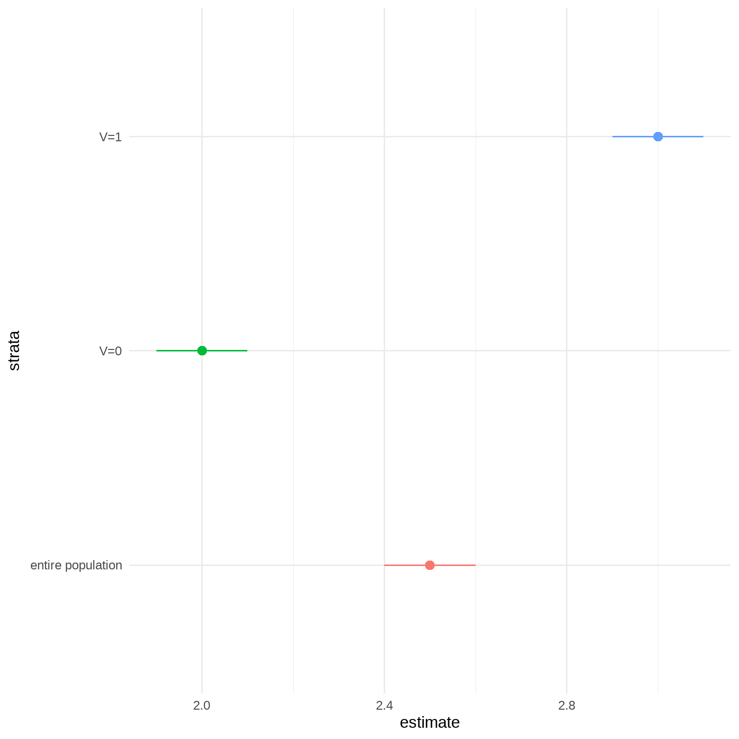
Conditional RR

$\frac{P r [Y = 1 | A = 1 | V = v]}{P r [Y = 1 | A = 0 | V = v]}$

## # A tibble: 1 x 3
##   V     term  estimate
##   <chr> <chr>    <dbl>
## 1 men   A         2.00

## # A tibble: 1 x 3
##   V     term  estimate
##   <chr> <chr>    <dbl>
## 1 women A         3.00

41 / 43

Conditional OR

$\frac{P r [Y = 1 | A = 1, V = v] / P r [Y = 0 | A = 1, V = v]}{P r [Y = 1 | A = 0, V = v] / P r [Y = 0 | A = 0, V = v]}$

## # A tibble: 1 x 3
##   V     term  estimate
##   <chr> <chr>    <dbl>
## 1 men   A         6.00

## # A tibble: 1 x 3
##   V     term  estimate
##   <chr> <chr>    <dbl>
## 1 women A         6.00

Average RR of 2.3 is between sex stratum-specific estimates of RR=2 for men and RR=3 for women
Average OR of 5.4 is smaller than sex stratum-specific estimates of OR=6 for men and OR=6 for women
OR is not collapsible in this example
Change in the conditional OR vs marginal OR due to non-collapsibility; exchangeability holds

42 / 43

Take home messagesEffect measure modification = effect heterogeneity
There's no the causal effect
Effect measure modifiers may or may not be proxies of the causal factors; no causal claims are made about effect measure modifiers
Do not confuse non-collapsibility with the lack of exchangeability
IPW and standardization are appropriate approaches for computing marginal causal effects in the entire population; stratification and matching are not
43 / 43

Definition of the effect modification

The causal effect changes with the characteristics of the population under study

greek_gods_po <- tibble::tribble( ~greek, ~V, ~Y_a0, ~Y_a1, "Rheia", 1, 0, 1, "Demeter", 1, 0, 0, "Hestia", 1, 0, 0, "Hera", 1, 0, 0, "Artemis", 1, 1, 1, "Leto", 1, 0, 1, "Athena", 1, 1, 1, "Aphrodite", 1, 0, 1, "Persephone", 1, 1, 1, "Hebe", 1, 1, 0, "Kronos", 0, 1, 0, "Hades", 0, 0, 0, "Poseidon", 0, 1, 0, "Zeus", 0, 0, 1, "Apollo", 0, 1, 0, "Ares", 0, 1, 1, "Hephaestus", 0, 0, 1, "Cyclope", 0, 0, 1, "Hermes", 0, 1, 0, "Dionysus", 0, 1, 0 )

↑, ←, Pg Up, k	Go to previous slide
↓, →, Pg Dn, Space, j	Go to next slide
Home	Go to first slide
End	Go to last slide
Number + Return	Go to specific slide
b / m / f	Toggle blackout / mirrored / fullscreen mode
c	Clone slideshow
p	Toggle presenter mode
t	Restart the presentation timer
?, h	Toggle this help

Effect modification

What If: Chapter 4

Elena Dudukina

2020-11-26

Definition of the effect modification

Definition of the effect modification

What is the average causal effect of A on Y in women and in men?

What is the average causal effect of A on Y in women and in men?

What is the average causal effect of A on Y in women and in men?

Results

Effect measure modification

Stratification to identify effect modification

Conditionally randomized "experiment"

Causal effect among romans

Causal effect among greeks

Results

Treatment effect in the treated

Computing the conditional risks

Surrogate vs causal effect modifier

Why care?

Additive vs multiplicative effect measure modification

Effect measure modification (EMM) vs interaction teaser

Stratification as adjustment

Matching as a form of adjustment

1:1 matching

Estimating different types of effects

Example

IPTW: average causal effect in the entire population

Stratification: sub-groups specific effects

1:1 Matching: treatment effect in the untreated or treated

Effect modification

Collapsibility

Non-collapsibility

RR

OR

Conditional RR

Conditional OR

Take home messages

Definition of the effect modification

Help